Unsupervised Machine Learning

Unsupervised machine learning is a class of techniques used to identify patterns, structures and groupings (clusters) within datasets. Crucially, unlike supervised machine learning, it does not require prior labelling.

There are two primary pillars of unsupervised machine learning: Clustering and Dimension Reduction.

Clustering Overview

• Clustering is a machine learning technique that groups data points based on similarities, applicable in scenarios like customer segmentation and market analysis.
• It can utilise one or multiple features to form meaningful clusters, aiding in exploratory data analysis and pattern recognition.

Types of Clustering Methods

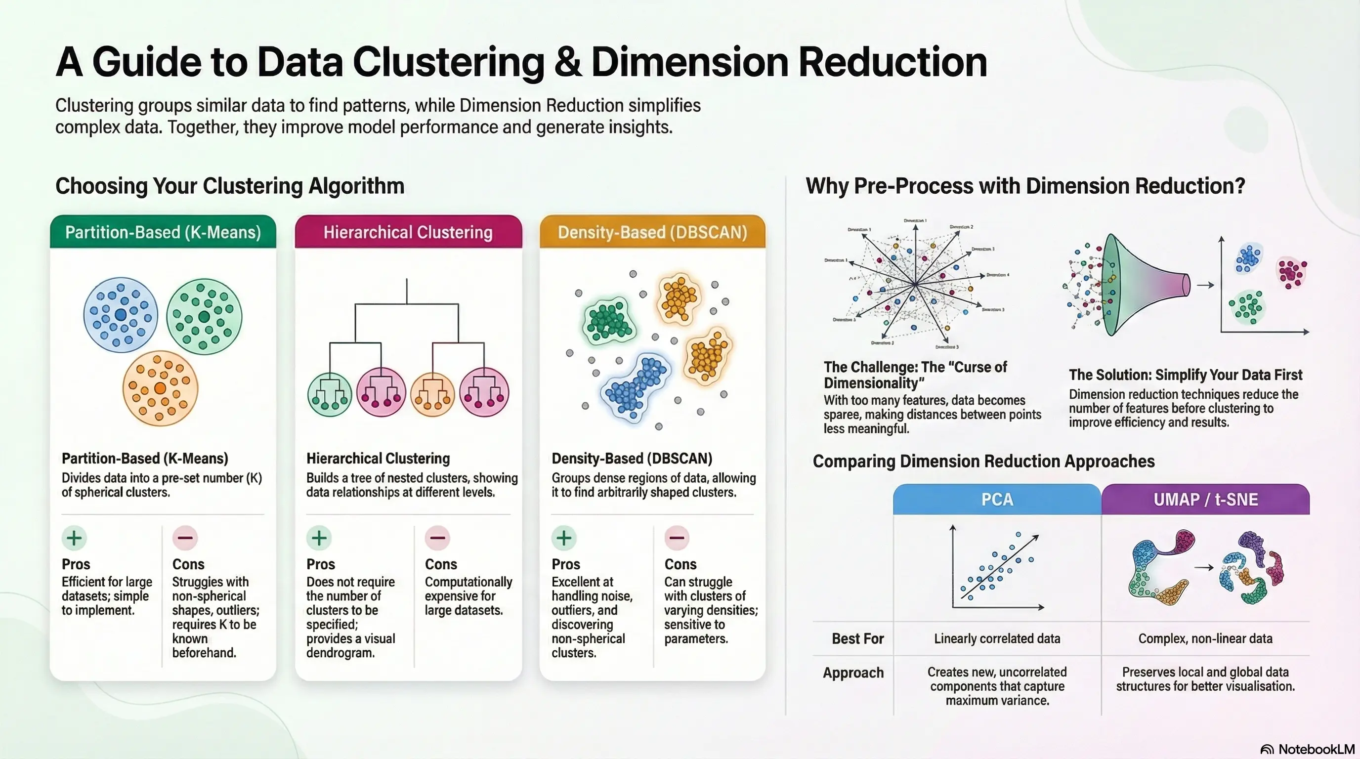
• Partition-based clustering, such as k-means, divides data into non-overlapping groups, optimising for minimal variance.
• Density-based clustering, like DBSCAN, identifies clusters of any shape, suitable for irregular and noisy datasets.
• Hierarchical clustering organises data into a tree structure, using agglomerative (bottom-up) and divisive (top-down) approaches to reveal relationships between clusters.

Applications of Clustering

The main purpose of clustering in machine learning is to group similar data points together based on their characteristics or features. This helps in identifying patterns and structures within the data without prior labeling. Key purposes include:

• Customer Segmentation: Identifying distinct groups of customers for targeted marketing.
• Anomaly Detection: Detecting outliers or unusual data points that may indicate fraud or errors.
• Data Summarisation: Reducing the complexity of data by summarising it into representative clusters.
• Exploratory Data Analysis: Uncovering natural groupings in data to gain insights and inform further analysis.

Clustering is essential for understanding the underlying structure of data and making informed decisions based on those insights.

The differences between k-means clustering and hierarchical clustering are as follows:

K-Means Clustering

• Method: A partition-based algorithm that divides data into a predefined number of clusters (k).
• Initialization: Requires the number of clusters (k) to be specified beforehand.
• Process: Iteratively assigns data points to the nearest cluster centroid and updates centroids until convergence.
• Scalability: Generally more efficient for large datasets, as it scales well with the number of data points.
• Shape of Clusters: Assumes spherical clusters and may struggle with non-globular shapes.

Hierarchical Clustering

• Method: Builds a hierarchy of clusters either through a bottom-up (agglomerative) or top-down (divisive) approach.
• Initialisation: Does not require the number of clusters to be specified in advance; the hierarchy can be cut at different levels to form clusters.
• Process: Creates a dendrogram that visually represents the merging or splitting of clusters based on distance metrics.
• Scalability: Less efficient for large datasets due to the computation of distance matrices, making it more suitable for smaller datasets.
• Shape of Clusters: Can identify clusters of various shapes and sizes, as it does not assume a specific cluster shape.

In summary, k-means is efficient for large datasets with a fixed number of clusters, while hierarchical clustering provides a more flexible approach to explore data relationships without prior specification of cluster numbers.

If you use k-means clustering on non-spherical clusters, several issues may arise:

• Poor Cluster Assignment: K-means assumes that clusters are spherical and evenly sized. If the actual clusters are elongated or irregularly shaped, k-means may incorrectly assign data points to the nearest centroid, leading to inaccurate clustering.

• Inaccurate Centroid Calculation: The algorithm calculates centroids based on the mean of the points in each cluster. For non-spherical clusters, this can result in centroids that do not represent the true center of the cluster, further distorting the clustering results.

• Overlapping Clusters: In cases where clusters overlap, k-means may struggle to separate them effectively, leading to mixed assignments and reduced cluster purity.

• Sensitivity to Initialization: The final clustering result can be heavily influenced by the initial placement of centroids. Poor initialization can lead to suboptimal clustering, especially in non-spherical distributions.

Overall, k-means is not well-suited for non-spherical clusters, and alternative clustering methods, such as density-based clustering (e.g., DBSCAN) or hierarchical clustering, may be more effective in such scenarios.

Non-spherical clusters

Non-spherical clusters are groups of data points that do not form a round or spherical shape when visualised. Instead, they can take on various forms, such as elongated, irregular, or even complex shapes. This is particularly important in clustering because many traditional clustering algorithms, like k-means, assume that clusters are spherical and evenly sized, which can lead to inaccurate results when dealing with real-world data.

To illustrate this concept, imagine a group of friends standing in a park. If they are all standing in a circle, that represents a spherical cluster. However, if they are scattered in a line or in a more complex formation, like a star shape, that represents a non-spherical cluster. Density-based clustering algorithms, such as DBSCAN, are often used to identify these non-spherical clusters because they can adapt to the shape of the data, allowing for more accurate grouping of points based on their density rather than their distance from a central point.

K-Means

The content focuses on K-Means Clustering, an iterative, centroid-based algorithm used to partition datasets into similar groups.

Understanding K-Means Clustering

• K-Means divides data into k non-overlapping clusters, where k is a chosen parameter, aiming for minimal variance around centroids and maximum dissimilarity between clusters.
• The centroid represents the average position of all points in a cluster, with data points closest to a centroid grouped together.

Using the K-Means Algorithm

• The algorithm starts by initializing k centroids, which can be randomly selected data points.
• It iteratively assigns points to the nearest centroid, updates centroids based on the mean of assigned points, and repeats until stabilization.

Challenges and Limitations

• K-Means struggles with imbalanced clusters and assumes clusters are convex and of similar sizes.
• It can perform poorly in the presence of noise and outliers, affecting the accuracy of clustering.

Determining the Optimal Number of Clusters (K)

• Choosing the right k is challenging; techniques like silhouette analysis, the elbow method, and the Davies-Bouldin index can help evaluate K-Means performance for different k values.

The main objective of the K-Means algorithm is to minimize the within-cluster variance for all clusters simultaneously. This means that the algorithm aims to ensure that data points within each cluster are as similar as possible (i.e., close to the centroid), while also maximizing the dissimilarity between different clusters.

In mathematical terms, this involves minimizing the sum of the squared distances between each data point and its corresponding cluster centroid.

In K-Means clustering, centroids play a crucial role as they represent the center of each cluster. Here are the key functions of centroids:

• Cluster Center: Each centroid is the average position of all data points assigned to that cluster. It serves as the reference point for the cluster.
• Assignment of Points: During each iteration, data points are assigned to the cluster whose centroid is nearest to them, based on a distance metric (usually Euclidean distance).
• Updating Centroids: After assigning points to clusters, the centroids are recalculated as the mean of all points in each cluster. This update process continues until the centroids stabilize and do not change significantly.

Overall, centroids are essential for defining the structure of the clusters and guiding the iterative process of the K-Means algorithm.

The distance matrix in K-Means clustering is significant for the following reasons:

• Point Assignment: It contains the distances between each data point and each centroid. This information is crucial for assigning each data point to the nearest centroid, determining which cluster it belongs to.
• Cluster Formation: By calculating the distances, the algorithm can effectively group data points into clusters based on proximity to centroids, ensuring that points within a cluster are closer to each other than to points in other clusters.
• Iteration Process: The distance matrix is recalculated in each iteration of the algorithm as centroids are updated. This allows the algorithm to adaptively refine cluster assignments and centroids until convergence is achieved.

Overall, the distance matrix is fundamental to the K-Means algorithm, enabling it to partition the dataset into meaningful clusters based on spatial relationships.

Determining the optimal value of K in K-Means clustering can be challenging, but several techniques can help:

1. Elbow Method:
   • Plot the sum of squared distances (inertia) for different values of K.
   • Look for the "elbow" point in the graph, where the rate of decrease sharply changes. This point suggests a suitable K value.
2. Silhouette Analysis:
   • Calculate the silhouette score for different K values, which measures how similar a data point is to its own cluster compared to other clusters.
   • A higher silhouette score indicates better-defined clusters, helping to identify the optimal K.
3. Davies-Bouldin Index:
   • This index evaluates the average similarity ratio of each cluster with its most similar cluster.
   • A lower Davies-Bouldin index indicates better clustering, guiding the selection of K.

Using these methods can provide insights into the most appropriate number of clusters for your dataset.

If K is set too high in K-Means clustering, several issues may arise:

• Overfitting: The algorithm may create clusters that are too specific, capturing noise and outliers rather than meaningful patterns in the data. This can lead to clusters that do not generalize well.

• Increased Complexity: More clusters can complicate the interpretation of results, making it harder to derive insights from the data. It may become challenging to understand the relationships between clusters.

• Centroid Proximity: As K increases, the centroids of clusters may become very close to each other, leading to clusters that are not distinct. This can result in poor separation between clusters.

• Diminishing Returns: Beyond a certain point, increasing K may not significantly improve the clustering quality, as the additional clusters may not provide valuable information.

If K is set too low in K-Means clustering, several problems may occur:

• Underfitting: The algorithm may group distinct data points into the same cluster, failing to capture the underlying structure of the data. This can lead to a loss of important information.

• Oversimplification: With too few clusters, the model may oversimplify the data, making it difficult to identify meaningful patterns or relationships among the data points.

• High Variance Within Clusters: Clusters may contain a wide range of data points that are not similar to each other, resulting in high variance within clusters. This can reduce the overall effectiveness of the clustering.

• Poor Interpretability: The resulting clusters may not be useful for analysis or decision-making, as they may not accurately represent the different groups present in the data.

DBSCAN and HDBSCAN Clustering

DBSCAN and HDBSCAN, which are used for density-based spatial clustering.

DBSCAN Overview

• DBSCAN (Density-Based Spatial Clustering of Applications with Noise) identifies clusters based on a user-defined density value around spatial centroids.
• It distinguishes between core points (with sufficient neighbors), border points (near core points but not dense enough), and noise points (isolated).

HDBSCAN Overview

• HDBSCAN (Hierarchical DBSCAN) is a variant that does not require parameter settings, making it more flexible and robust against noise.
• It uses cluster stability to adaptively adjust neighborhood sizes, resulting in more meaningful clusters.

Comparison and Applications

• DBSCAN is not iterative and grows clusters in one pass, while HDBSCAN builds a hierarchy of clusters based on varying densities.
• HDBSCAN often identifies more distinct clusters and handles complex data patterns better than DBSCAN.

The main differences between DBSCAN and HDBSCAN are:

• Parameter Requirement:

  • DBSCAN requires the user to set two parameters: the minimum number of points (n) in a neighborhood and the radius (epsilon) for defining neighborhoods.
  • HDBSCAN does not require these parameters to be set, making it more user-friendly and flexible.

• Cluster Stability:

  • DBSCAN identifies clusters based on fixed density criteria and does not adapt to varying densities in the data.
  • HDBSCAN uses cluster stability, which allows it to adaptively adjust the neighborhood size based on local density variations, resulting in more robust clusters.

• Handling Noise:

  • DBSCAN can label points as noise if they do not belong to any cluster.
  • HDBSCAN is generally less sensitive to noise and can produce more meaningful clusters in the presence of outliers.

These differences make HDBSCAN more effective in complex datasets with varying densities and noise.

In DBSCAN, a core point is defined as a point that has at least a specified minimum number of neighboring points (including itself) within a given radius (epsilon). Specifically:

• Core Point Criteria:
  • A point is considered a core point if it has at least n points (the minimum number of points parameter) within its neighborhood defined by the radius epsilon.

Core points are essential for forming clusters, as they serve as the focal points from which clusters are expanded by including their neighboring points.

In DBSCAN, border points play a crucial role in the clustering process:

• Definition: A border point is a point that falls within the neighborhood of a core point but does not have enough neighboring points to qualify as a core point itself.

• Role:

  • Cluster Inclusion: Border points are included in the same cluster as their associated core points. They help to extend the boundaries of the cluster.
  • Less Dense Connection: While they belong to a cluster, border points are not as densely connected as core points, meaning they are on the outer edges of the cluster.

Overall, border points help define the shape and extent of clusters while indicating areas where the density of points decreases.

HDBSCAN, which stands for Hierarchical Density-Based Spatial Clustering of Applications with Noise, is an advanced clustering algorithm that builds upon the principles of DBSCAN. Unlike its predecessor, HDBSCAN does not require you to set specific parameters, making it more user-friendly and adaptable to various data sets. Imagine trying to find groups of friends in a crowded room without knowing how many groups there are; HDBSCAN helps you do just that by automatically adjusting to the density of the crowd.

Here's how it works: HDBSCAN starts by treating each data point as its own cluster, similar to how you might initially see every person in the room as an individual. It then gradually merges these clusters based on their density, creating a hierarchy of clusters. This process allows HDBSCAN to identify clusters of varying shapes and sizes, even in the presence of noise or outliers. The result is a more coherent and meaningful representation of your data, where clusters are defined not just by their proximity but also by their stability across different density levels.

Clustering, Dimension Reduction, and Feature Engineering

Clustering Techniques

• Clustering aids in feature selection and creation, enhancing model performance and interpretability.
• It helps identify similar or correlated features, allowing for the selection of representative features and reducing redundancy.

Dimension Reduction

• Dimension reduction simplifies data structures, making it easier to visualize high-dimensional data and improving computational efficiency.
• Techniques like PCA, t-SNE, and UMAP are used to reduce dimensions before clustering, which enhances the effectiveness of clustering algorithms.

Application in Face Recognition

• Dimension reduction is applied in face recognition using eigenfaces, where PCA extracts key features from a dataset to improve prediction accuracy.
• This process minimizes computational load while preserving essential features for identifying faces, demonstrating the practical application of these techniques.

Principal Component Analysis (PCA) plays a crucial role in dimension reduction by transforming high-dimensional data into a lower-dimensional space while preserving as much variance as possible. Here are the key points regarding PCA's role:

• Feature Extraction: PCA identifies the directions (principal components) in which the data varies the most. These components are linear combinations of the original features.
• Variance Preservation: By selecting the top principal components, PCA retains the most significant variance in the data, which helps maintain the essential characteristics of the dataset.
• Noise Reduction: By reducing dimensions, PCA can help eliminate noise and redundant features, leading to improved model performance.
• Visualization: PCA simplifies the visualization of high-dimensional data by projecting it into two or three dimensions, making it easier to interpret and analyze.

In summary, PCA is a powerful technique for reducing the complexity of data while retaining its important information, making it a valuable preprocessing step in machine learning tasks.

Clustering plays a significant role in feature selection by helping to identify and group similar or correlated features. Here are the key points regarding its significance:

• Redundancy Reduction: Clustering allows you to group features that provide similar information. By selecting a representative feature from each cluster, you can reduce redundancy and simplify the dataset.

• Improved Model Performance: By eliminating redundant features, clustering can enhance model performance by reducing overfitting and improving generalization.

• Feature Interaction Identification: Clustering can reveal interactions between features, helping to identify which features work well together and may be important for predictive modeling.

• Dimensionality Reduction: By selecting fewer, more informative features based on clustering, you can effectively reduce the dimensionality of the dataset, making it easier to analyze and visualize.

In summary, clustering aids in feature selection by simplifying the feature space, enhancing model performance, and providing insights into feature relationships.

Clustering can significantly enhance feature engineering decisions in the following ways:

• Identifying Subgroups: Clustering helps identify distinct subgroups within the data. Understanding these subgroups can guide the creation of new features that capture specific interactions or characteristics relevant to each group.
• Feature Transformation: By analyzing clusters, you can determine which transformations (e.g., scaling, encoding) may be beneficial for specific features, leading to more effective modeling.
• Reducing Feature Space: Clustering allows you to select representative features from each cluster, reducing the overall number of features while preserving valuable information. This simplification can lead to more efficient models.
• Enhancing Interpretability: Clustering can provide insights into the relationships between features, making it easier to interpret the model and understand how different features contribute to predictions.

In summary, clustering aids in making informed feature engineering decisions by revealing patterns, guiding transformations, and simplifying the feature space, ultimately leading to better model performance and interpretability.

If you don't reduce dimensions before clustering, several challenges may arise:

• Curse of Dimensionality: As the number of dimensions increases, the volume of the space increases exponentially, making data points sparse. This sparsity can lead to less meaningful distances between points, making clustering less effective.
• Increased Computational Complexity: High-dimensional data requires more computational resources for clustering algorithms, which can slow down processing and make it less feasible to work with large datasets.
• Difficulty in Visualization: Clustering results in high-dimensional spaces are hard to visualize, making it challenging to interpret the clusters and understand the underlying patterns in the data.
• Overfitting: Clustering in high dimensions can lead to overfitting, where the model captures noise rather than the underlying structure of the data, resulting in poor generalization to new data.

In summary, not reducing dimensions before clustering can lead to ineffective clustering results, increased computational demands, and difficulties in interpretation and visualization.

Dimension Reduction Algorithms

Dimension Reduction Algorithms are essential for simplifying high-dimensional datasets while preserving critical information.

Dimension Reduction Algorithms

• These algorithms reduce the number of features in a dataset, making it easier to analyze and visualize.
• Key algorithms include Principal Component Analysis (PCA), T-Distributed Stochastic Neighbor Embedding (t-SNE), and Uniform Manifold Approximation and Projection (UMAP).

Principal Component Analysis (PCA)

• PCA is a linear method that transforms features into uncorrelated variables called principal components, retaining maximum variance.
• It effectively reduces noise and dimensionality while maintaining essential information.

T-Distributed Stochastic Neighbor Embedding (t-SNE) and UMAP

• t-SNE maps high-dimensional data to lower dimensions, focusing on preserving local similarities but struggles with scalability and tuning.
• UMAP, an alternative to t-SNE, constructs a high-dimensional graph and optimizes a low-dimensional representation, often providing better clustering performance and scalability.

If PCA fails or is not suitable for your data, you can consider the following alternative dimensionality reduction methods:

1. T-Distributed Stochastic Neighbor Embedding (t-SNE):
   • Focuses on preserving local similarities in high-dimensional data.
   • Effective for visualizing complex datasets, especially in two or three dimensions.
   • However, it may struggle with scalability and requires careful tuning of hyperparameters.
2. Uniform Manifold Approximation and Projection (UMAP):
   • Constructs a high-dimensional graph representation of the data and optimizes a low-dimensional structure.
   • Preserves both local and global data structures, often providing better clustering performance than t-SNE.
   • Generally scales better than t-SNE and is suitable for larger datasets.

These methods can be particularly useful when dealing with non-linear relationships in the data that PCA may not capture effectively.

Python K-means Clustering
Python Comparing DBSCAN and HDBSCAN
Python Principle Component Analysis (PCA)
Python t-SNE and UMAP